How to Calculate Loan Amortisation Schedules Using Excel

Loan amortisation is a critical process for managing debt, whether it's a mortgage, car loan, or personal loan. A Loan Amortisation Schedule breaks down each payment into principal and interest portions, helping borrowers understand how their payments are applied over time. This detailed insight aids in planning finances and exploring early repayment strategies.

In this blog, we’ll walk through the process of creating a loan amortisation schedule using Excel, making it easy for you to track payments and understand your loan better.

What is Loan Amortisation?

Loan Amortisation involves repaying a loan through fixed payments over a set term. Each payment consists of two parts:

• Principal Repayment: Reduces the outstanding loan balance.
• Interest Payment: The cost of borrowing, calculated on the remaining balance.

Key Elements of Loan Amortisation:

1. Principal (P): The original amount borrowed.
2. Interest Rate (r): The annual interest rate charged on the loan.
3. Term (n): The total time period of the loan, usually in months.
4. Monthly Payment (PMT): A fixed amount paid each month.

Monthly Payment Formula:

PMT = [P × r × (1 + r)^n] / [(1 + r)^n - 1]

Where:

• PMT = Monthly Payment
• P = Principal (Loan amount)
• r = Monthly interest rate (annual rate / 12)
• n = Total number of payments (months)

Step-by-Step Guide: Building an Amortisation Schedule in Excel

Excel simplifies the process of creating a loan amortisation schedule with the PMT function and other formulas. Follow these steps to build a complete schedule:

Step 1: Calculate Monthly Payment Using the PMT Function

PMT Function:
Excel
Copy code
=PMT(rate, nper, pv, [fv], [type])

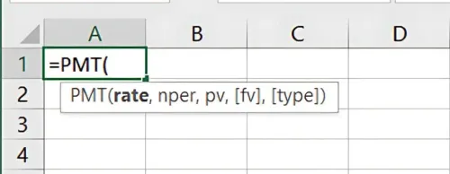
• rate: Monthly interest rate (annual rate/12).
  
• nper: Total number of periods (term in months).
  
• pv: Present value or principal (loan amount).
  
• fv: Future value (optional, usually 0 for fully paid loans).
  
• type: Payment timing (0 for end of period, optional).
  

Example Calculation: For a ₹10,000 loan at a 6% annual interest rate over 24 months:
Excel
Copy code
=PMT(0.06/12, 24, -10000)

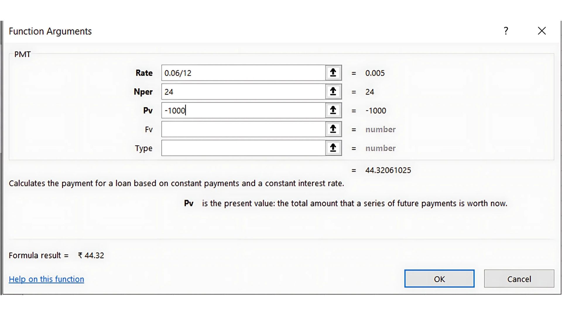
Result: -443.21 This means the monthly payment is ₹443.21.

Step 2: Set Up Amortisation Table

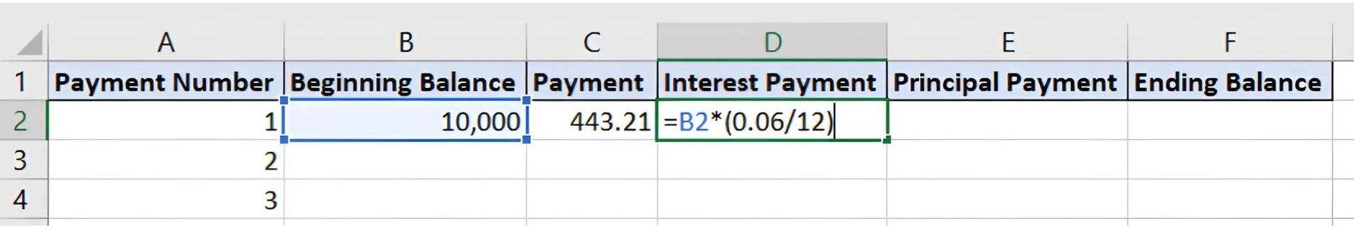
1. Create Columns:

• Column A: Payment Number (1, 2, 3, ...)
• Column B: Beginning Balance
• Column C: Payment
• Column D: Interest Payment
• Column E: Principal Payment
• Column F: Ending Balance
  

2. Enter the Principal and Monthly Payment:
   

• B2: Enter the loan amount (e.g., ₹10,000).
• C2: Enter the calculated PMT value (e.g., 443.21).
  

3. Calculate the Interest and Principal Portions:
   D2 (Interest Payment):
   

=B2 * (0.06/12)

E2 (Principal Payment):
=C2 - D2

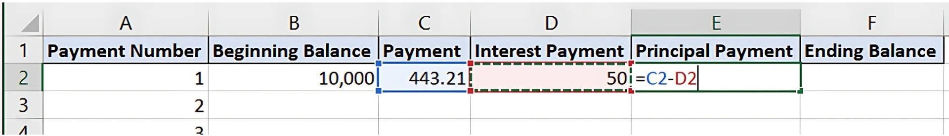
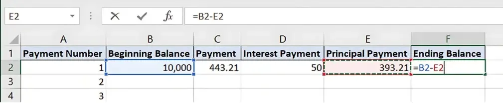
4. Calculate the Ending Balance:

F2 (Ending Balance):
=B2 - E2

5. Copy Formulas Down the Rows: Copy the formulas for interest, principal, and ending balance down the rows. Use the ending balance from one period as the beginning balance for the next.

Step 3: Complete the Amortisation Table

Continue copying formulas until the ending balance reaches zero. This table will display a detailed breakdown of each payment, how much goes toward interest, and how much reduces the loan balance.

This schedule helps you see how each payment is divided between interest and principal, making it easy to track progress and plan for early repayments.

Benefits of Using an Amortisation Schedule

• Financial Clarity: Understand how much of each payment goes toward interest versus reducing the principal.
• Early Payoff Planning: Helps you strategise for paying off your loan faster.
• Better Decision-Making: Knowing the breakdown of payments can assist in comparing different loan options.

Key Takeaways:

• Loan Amortisation divides payments into principal and interest, providing a clear roadmap for repayment.
• The PMT function in Excel simplifies calculating monthly payments.
• An Amortisation Schedule offers a detailed view of how each payment impacts your loan balance, making it a valuable tool for financial planning.

Conclusion:

Building an Amortisation schedule in Excel allows you to manage loan repayments efficiently. It offers a transparent view of each payment and helps in planning for future financial goals.

Next Chapter Preview: In the next chapter, we will explore EMI (Equated Monthly Installment) Calculation for Loans and Mortgages, focusing on understanding the EMI formula, factors that affect EMI, and step-by-step calculations in Excel. Stay tuned to learn how to handle monthly payments more effectively!